Fernandez Thermal Storage

[fernandez]

Hope everyone is having a good week!

This week, I’ve been taking a look at aluminium thermal storage sizing. As discussed at last week’s research meeting, we want the thermal storage to be ready to boil water after about 4 hours of heating at 100W. This should cover the use case where someone wants to cook lunch on the ISEC and then have their thermal storage be ready for dinner time.

Using 4 hours as a baseline and heat loss of 1W per 10 C, I was able to determine that the ideal mass of the thermal storage was around 3.5 - 4kg. At that mass, we could boil around 2.5L of water, which is a considerable amount! Based on the dimensions’s of Bidjanga’s proposed thermal storage, it would weigh just under 4kg which is right where we want it to be.

The last thing to consider would be the flux supplied to the water, which would be a function of the contact area and thermal conductivity between the pot and the thermal storage. The larger the contact area, the higher we would expect the flux to be (which means we would heat food faster). That being said, making the pot bigger would increase the surface area on the top of the thermal storage for heat to be lost (towards the lid). In addition, we need to think about the user experience; how large of a pot is too large for someone to realistically use and have in their kitchen/workspace? As we increase the diameter, the footprint will also increase.

My Python thermal simulation development is currently blocked until I figure out how to handle the boundary condition at the thermal interface. In the meantime, I am looking using a 3D modeling software like SolidWorks or Fusion360 to accomplish the same thing at a higher fidelity. The only blocker there is licensing. SolidWorks used to be free through the university and I have used it extensively, but my license has expired. Fusion looks like they have a free option which I will explore this evening.

[fernandez]

Hey Everyone,

Last week, I shifted over to using SolidWorks for Thermal Modeling. SolidWorks is a 3D modeling tool that has simulation models included for heat transfer; making our lives a lot easier. The only downside to using Solidworks is that itteration will be a bit more time consuming.

This week, I am trying to:

• Get familiar with SolidWorks Simulation
• Answer how the heat flux between the thermal storage and the food varies with the temperature of the two substances.

I’ve made some good progress with the first objective. I started by modeling a cylindrical aluminium thermal storage with one litre of water directly above it. The screenshot below illustrates the described configuration in the 3D modelling software, SolidWorks.

Once the model was created, I started playing with SolidWork’s Thermal Study tool to analyze how heat transfered between the aluminium and the water using the same configuration described above.

I ran a simulation with the following parameters:

Duration: 2 Hours (7200 seconds)
Step Size: 10 Seconds

Below is a screenshot of the model’s temperature distribution after the first time step (10 seconds into the simulation).

The temperature gradient shows heat moving from the hotter aluminium thermal storage up into the water that we are trying to boil. Within the first few seconds of the simulation, the water heats significantly; reaching 50 C within the first 10 seconds.

Around 11 minutes into the simulation, all of the water reaches 100 C (boils), as can be seen below. Keep in mind that the scale of the gradient changes from plot one to plot 2. Unfortunately, there is no option to make the legend bigger for this view.

Although I am still working to validate the simulation, this result seems reasonable considering the large surface area of heat transfer and perfect conduction. Because I do not simulate convective effects yet, the cold water remains on the top of the model. If the liquid was stired as it was placed in contact with the aluminium, I would expect the water to boil even faster. Additionally, I need to investigate how Solidworks handles phase changes, given some of the water in the model reaches well over boiling temperature.

The simulation also allowed me to investigate the heat flow accross the thermal interface of the aluminium and water, however further work needs to be done to both validate and present the data in a more digestable fashion. Expect more results in the coming days.

[fernandez]

Hi Everyone!

This week I have been working on a few things:

• Adding Pot and Lid to Model
• Adding Convection to Thermal Simulation

I started by adding a pot and lid to the model in order to enclose the heat sink (water in this case).
I used very similar parameters to the previous simulation, with a 5kg thermal storage and 1 litre of water.

A section view of the configuration is below to illustrate the cavity where the water is situated.

Using SolidWork’s Flow Simulation tool, I set up a convective heat transfer simulation assuming the following:

• Thermal Storage Starts at 300 C
• Water Starts at 20 C
• System is adiabatic (perfectly insulated; no energy enters or leaves)
• Pot and Thermal Storage are connected (perfectly conducting)

Below are two views of the fluid velocities after 60 seconds of simulation. The legend indicates the velocity of the fluid. As expected, higher enery molecules rise to the top of the model before falling back down to the bottom of the pot, getting heated, and rising up again.

This first illustration shows a near top-down view of the pot of water with the lid removed for viewing purposes.

This second illustration shows a side view of the flow in a section view so that the flow is more easily visible.

The above illustrations validate that convection is, indeed, working as expected in the model. The convecting model significantly increases the rate at which the water boils. The configuration presented, for example, boils a litre of water in about 70 seconds.

A video of the thermal simulation is presented below, with an included temperature gradient. Note that the minimum and maximum temperatures of the gradient change as the simulation is run, so please monitor the legend to understand the temperature profile. The simulation illustrates a static side-view slice of the model.

Link to Thermal Simulation Video

Next week, I intend to take a look into adding an air gap to the model. This will also allow me to experiment with adding insulation to the unit and simulating it more realistically with losses due to air convection, for example. The above simulation mode assumes an interior flow whereas an air gap between the pot and the thermal storage is an external flow. This is a key disticntion in the modelling software.

Thanks and let me know if you have any questions!

[fernandez]

Hey everyone,

I was on vacation last week for Vetran’s day so I appoligize for not posting.

I’ve been working on adding external convective effects to the model to mimic air flow around the ISEC which is where (likely) most of our losses will occur.

To facilitate this, I upgraded the model to include both the glass-fiber insulation and an aluminium container. I modeled the geometry of the ISEC using rough measurement’s I took from the ISEC I brought home from Cal Poly; about a foot and a half tall and a foot and a half in diameter.

A cut view of the model illustrates the configuration of the ISEC. The glassfiber insulation was arranged with a wall thickness of 4.25 inches (from Cal Poly ISEC) and floor and lid thicknesses of around 7 and 2 inches respectively.

In order to simulate external air flow, I set up a computational domain around the ISEC. The computational domain was then filled with air while the ISEC’s cooking cavity was filled with water.
Due to limitations in the simulation software, liquid water and gaseous air could not be simulated in the same enclosed cavity. To better simulate our ISEC’s operational configuration, an air cavity was placed on top of the cooking vessel to simulate the semi-stagnant air that is trapped in the pot during normal operation. The computational domain is illustrated below.

The screenshot below illustrates the flow lines for a cross section of the ISEC after 10 minutes of heat exchange. The water (red) visibly wicks away most of the heat from the thermal storage with the air column (light blue) on top of the water leeching heat as well. As expected, the insulation does a good job of maintaining the external surface of the ISEC at room temperature; limiting losses from external convection. That being said, some energy is lost to heating the insulation surrounding the puck.

Although I had aimed to complete this last week, over the next week I will be playing with adding an air gap between the pot and the thermal storage and seeing how that effects the rate at which heat is dumped from the thermal storage to the water in the pot. In addition, I will try to quantify the conductive losses between the thermal storage and the insulation as well as the convective losses from airflow around the container.

Thanks and let me know if you have any questions or comments.

Best,

Michael

[fernandez]

Hey everyone!

Over the last few weeks, between eating turkey and pumpkin pie, I’ve been looking into the thermal interface between our thermal storage (an aluminium puck) and our heat sink (a pot with water in it).

The junction between the two materials is pivitol to the model that is being developed as its properties determine how much heat flows from the thermal storage device and the water that we are trying to heat. The junction has been difficult to model because there are many real-world attributes such as the surface roughness of the interface that are challenging to quantify and implement in a software solution.

As disucssed last week, I began by experimenting with how an air gap effects the boiling time of 2 litres of water in the simulation described in the previous post (insulated with convection). The air gap between the conducting surfaces is plotted on the X-Axis alongside the time it took for the 2 litres of water to reach 100C on the Y-Axis. Without any air gap, the water boiled in about 5.5 minutes. Adding a tiny air gap of just 0.1 micrometers nearly doubled the boiling time to roughly 10 minutes. Additional increases in air gap increased the boiling time to a lesser extent, but the effect was still apparent.

Although this information was promising, I had a feeling that there must be a better way to quantify and model the imperfection of the thermal interface. After chatting with a coworker, it turns out that there is a parameter known as the thermal contact resistance of an interface that describes such imperfections. Thankfully, Solidwork’s Flow Simulation tool allows you to specify the contact resistance of the interface and model the heat exchange between the two solids. Unfortunately, the parameter is something that must be measured experimentally, as it accounts for a wide range of inputs.

Solidworks defines the contact resistance with units of (kelvin*meter^2)/watt giving a ground aluminium surface with a roughness of 2.5 micron a contact resistance of 8.8 e-5K*m^2/W; inverting the parameter to make it a bit more transparent, 11 kW/m^2*K. That is, for a square meter of surface area, the heat flux accross the surface increases by 11 kW for every degree of temperature difference accross the gap.

A few weeks ago, Andrew S. perfomed an experiment to see how fast he could boil a litre of water with a 3.2 kg aluminium thermal storage heated to 350 C. In his experiment (shown below), he was able to boil the water in a bit over 20 minutes. The first litre is removed and second placed in the pot once the first litre reaches 100 C.

Out of curiosity, I replicated Andrew’s experimental setup in Solidworks using puck and pot geometry that he provided to me. Using the contact resistance preset described above, 1 litre of water boiled in 3 minutes; significantly faster than the experiment that was ran. This told me that the contact resistance of the actual junction is significantly different than the Solidwork’s preset I used in the simulation.

Using the experimental data from Andrew’s test, I have attempted to estimate the contact resistance for use in the simulation. Although still a work in progress, initial results are promising when evaluating the first 20 minutes of the experiment. Below is a 10 second running average of the instantaneous contact resistance for the interface.

Based on the results above, I chose a conservative value of 270 W/Km^2 (0.00369 Km^2/W) for the next Solidworks simulation. The simulation ran for much longer time, taking over 15 minutes for the water to reach 100 C; much closer to the 20 minutes it took in the experiment. The results are below.

While this analysis is by no means complete, I think I have a lot better understanding of how the interface between the thermal storage and the pot of water behaves and specifically how to model and characterize it based on experimental data.

[fernandez]

It’s been a while since I posted to this forum but with the new quarter in full swing, I’ve got some updates to share. Last quarter, I focused mostly on analysis and understanding the thermal properties of our ISEC system. This quarter, I am trying to focus more on experimentation, particularly with regards to the solid thermal storage (STS) and pot interface. The STS-Pot interface seems to be a particularly important interface that we need to make sure is conducting heat efficiently; allowing us to cook food rapidly.

To facilitate this, I have been working on procuring and installing STS into my existing ISEC.

Together with the STS mechanical team, we took a foot long section of extruded aluminium 6061 alloy roughly 6.25 inches in diameter and sectioned it into large sections. Roughly 6 and 8kgs respectively. I took the heavier one, which still must be measured precisely, but is roughly 8kg.

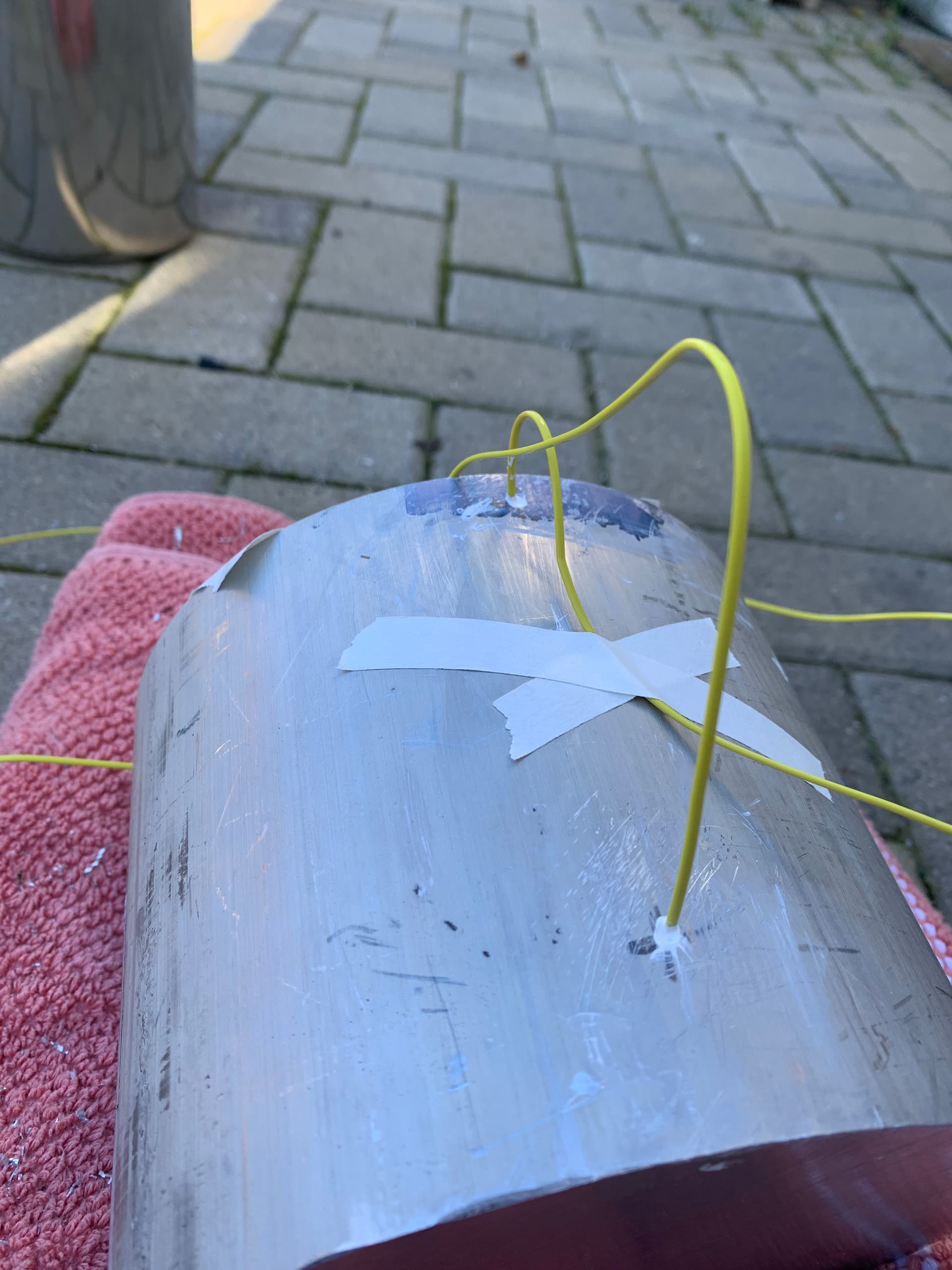
To measure the temperature of the ISEC during testing, I decided to install two Type K thermal couples to the STS. Wanting to have a secure connection that is repesentaive of the internal temperature of the ISEC, I opted to drill two holes, approximately 1 inch in depth, into the ISEC.

I then filled the holes with a non-electrically-conductive thermal paste rated for high temperature applications to ensure good thermal contact between the aluminium and the thermocouple. After ensuring the holes were packed full of paste, I inseted the thermocoulples and secured them in place with masking tape temporarily while I worked on mixing some epoxy.

I opted to use JB Weld Steel Cold Solder which is rated for a continuous use temperature of over 500C. Once I applied the epoxy, I let it cure overnight at room temperature.

---

The next morning I wanted to put the thermal storage to work to make sure that the thermisters were working as expected. It was a cold morning but bright morning with the thermal storage starting at 10C.

In this test, I hooked a 100W solar panel to a classic ISEC pancake heater and placed the 8kg aluminium thermal storage directly on top with no additional modification. This test was meant to be a baseline before I begin making improvements to the design.

I hooked the thermister closest to the pancake heater to channel 0 of the datalogger and hooked the other to channel 1.

I left the ISEC out in the sun for a bit over 2 hours, rotating it periodically to maintain a sun-pointing configuration. I set the datalogger to record data every 30 seconds and at the end of the two hour period, the STS had reached nearly 70C, indicating we were getting roughly 60W of net power into the STS throughout the period.

Over the next few days, I worked on piecing together a python script to handle parsing the data coming from the datalogger and streamlining processing. The python script currently parses the data and produces two sets of plots: temperature versus time and the rate of change in temperature as a function of time. It produces these plots for each channel. Although the test only used two channels, four channels will be used in the near future when I attempt to heat a pot of water.

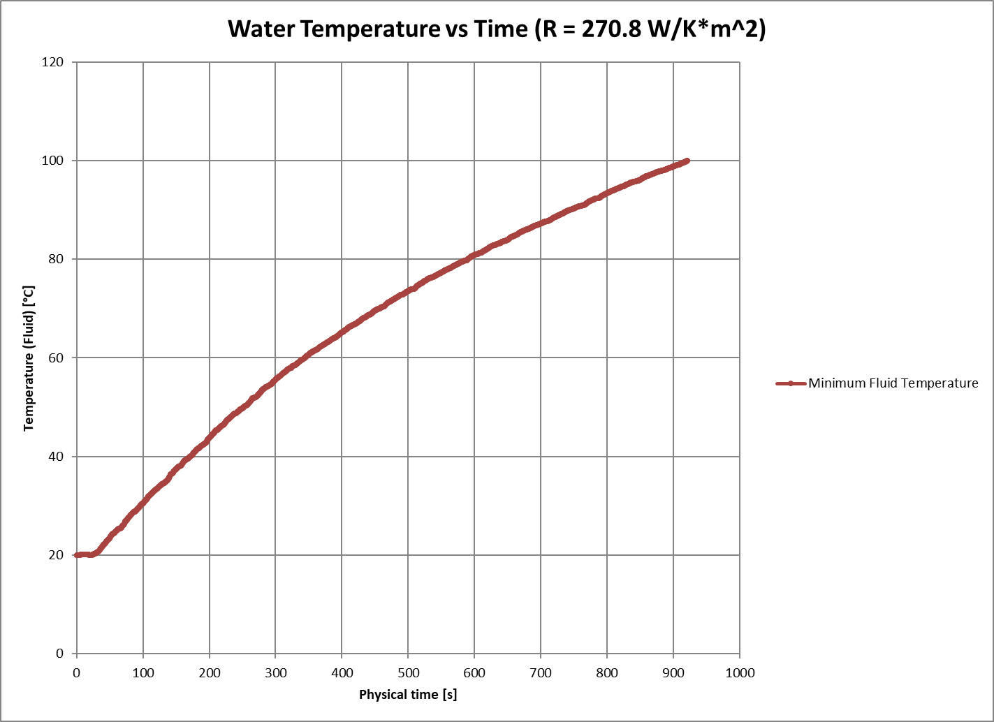
Below are the results from this test:

From this test I’ve learned the following:

• Both thermocouples report very similar temperatures throughout the entire test because the rate of heating the STS is much slower than the inter-STS heat transfer. In effect, the entire STS heats up at the same rate.
• The connection between the heater and the STS can likely be improved as we were getting around 50% of the power to the STS that we were expecting. Of course, there are other losses such as pointing losses, STS heat losses, and inefficiency of the heater itself (not converting 100% of the input power to heat)
• The datalogger works as expected and I have a repeatable way to produce metrics like the ones above
• More power would make future tests a lot faster and would let me itterate quicker

Overall, a really fun week of testing.

Moving forward I’m going to install a thermal pad at the STS-heater interface to see if it improves the rate at which we heat the ISEC. I’m also going to start experimenting with the STS-Pot interface.